Layer-Wise Learning Rate in PyTorch
Implementing discriminative learning rate across model layers


Last update: 29.03.2022. All opinions are my own.
1. Overview
In deep learning tasks, we often use transfer learning to take advantage of the available pre-trained models. Fine-tuning such models is a careful process. On the one hand, we want to adjust the model to the new data set. On the other hand, we also want to retain and leverage as much knowledge learned during pre-training as possible.
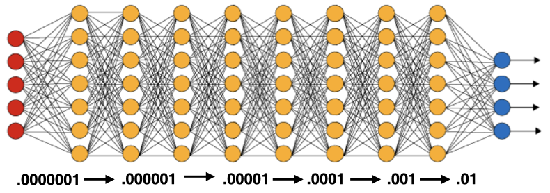
Discriminative learning rate is one of the tricks that can help us guide fine-tuning. By using lower learning rates on deeper layers of the network, we make sure we are not tempering too much with the model blocks that have already learned general patterns and concentrate fine-tuning on further layers.
This blog post provides a tutorial on implementing discriminative layer-wise learning rates in PyTorch. We will see how to specify individual learning rates for each of the model parameter blocks and set up the training process.
2. Implementation
The implementation of layer-wise learning rates is rather straightforward. It consists of three simple steps:
- Identifying a list of trainable layers in the neural net.
- Setting up a list of model parameter blocks together with the corresponding learning rates.
- Supplying the list with this information to the model optimizer.
Let's go through each of these steps one by one and see how it works!
2.1. Identifying network layers
The first step in our journey is to instantiate a model and retrieve the list of its layers. This step is essential to figure out how exactly to adjust the learning rate as we go through different parts of the network.
As an example, we will load one of the CNNs from the timm library and print out its parameter groups by iterating through model.named_parameters() and saving their names in a list called layer_names. Note that the framework discussed in this post is model-agnostic. It will work with any architecture, including CNNs, RNNs and transformers.
# instantiate model
import timm
model = timm.create_model('resnet18', num_classes = 2)

# save layer names
layer_names = []
for idx, (name, param) in enumerate(model.named_parameters()):
    layer_names.append(name)
    print(f'{idx}: {name}')
As the output suggests, our model has 62 parameter groups. When doing a forward pass, an image is fed to the first convolutional layer named conv1, whose parameters are stored as conv1.weight. Next, the output travels through the batch normalization layer bn1, which has weights and biases stored as bn1.weight and bn1.bias. From that point, the output goes through the network blocks grouped into four big chunks labeled as layer1, ..., layer4. Finally, extracted features are fed into the fully connected part of the network denoted as fc.
In the cell below, we reverse the list of parameter group names to have the deepest layer in the end of the list. This will be useful on the next step.
# reverse layers
layer_names.reverse()
layer_names[0:5]
2.2. Specifying learning rates
Knowing the architecture of our network, we can reason about the appropriate learning rates.
There is some flexibility in how to approach this step. The key idea is to gradually reduce the learning rate when going deeper into the network. The first layers should already have a pretty good understanding of general domain-agnostic patterns after pre-training. In a computer vision setting, the first layers may have learned to distinguish simple shapes and edges; in natural language processing, the first layers may be responsible for general word relationships. We don't want to update parameters on the first layers too much, so it makes sense to reduce the corresponding learning rates. In contrast, we would like to set a higher learning rate for the final layers, especially for the fully-connected classifier part of the network. Those layers usually focus on domain-specific information and need to be trained on new data.
The easiest approach to incorporate this logic is to incrementally reduce the learning rate when going deeper into the network. Let's simply multiply it by a certain coefficient between 0 and 1 after each parameter group. In our example, this would gives us 62 gradually diminishing learning rate values for 62 model blocks.
Let's implement it in code! Below, we set up a list of dictionaries called parameters that stores model parameters and learning rates.
We will simply go through all parameter blocks and iteratively reduce and assign the appropriate learning rate.
In our example, we start with lr = 0.01 and multiply it by 0.9 at each step.
Each item in parameters becomes a dictionary with two elements:
-
params: tensor with the model parameters -
lr: corresponding learning rate
# learning rate
lr      = 1e-2
lr_mult = 0.9

# placeholder
parameters = []

# store params & learning rates
for idx, name in enumerate(layer_names):

    # display info
    print(f'{idx}: lr = {lr:.6f}, {name}')

    # append layer parameters
    parameters += [{'params': [p for n, p in model.named_parameters() if n == name and p.requires_grad],
                    'lr':     lr}]

    # update learning rate
    lr *= lr_mult
As you can see, we gradually reduce our learning rate from 0.01 for the bias on the classification layer to 0.00001 on the first convolutional layer. Looks good, right?!
Well, if you look closely, you will notice that we are setting different learning rates for parameter groups from the same layer. For example, having different learning rates for fc.bias and fc.weight does not really make that much sense. To address that, we can increment the learning rate only when going from one group of layers to another. The cell below provides an improved implementation.
#collapse-hide

# learning rate
lr      = 1e-2
lr_mult = 0.9

# placeholder
parameters      = []
prev_group_name = layer_names[0].split('.')[0]

# store params & learning rates
for idx, name in enumerate(layer_names):

    # parameter group name
    cur_group_name = name.split('.')[0]

    # update learning rate
    if cur_group_name != prev_group_name:
        lr *= lr_mult
    prev_group_name = cur_group_name

    # display info
    print(f'{idx}: lr = {lr:.6f}, {name}')

    # append layer parameters
    parameters += [{'params': [p for n, p in model.named_parameters() if n == name and p.requires_grad],
                    'lr':     lr}]
This looks more interesting!
Note that we can become very creative in customizing the learning rates and the decay speed. There is no fixed rule that always works well. In my experience, simple linear decay with a multiplier between 0.9 and 1 is a good starting point. Still, the framework provides a lot of space for experimentation, so feel free to test out your ideas and see what works best on your data!
2.3. Setting up the optimizer
We are almost done. The last and the easiest step is to supply our list of model parameters together with the selected learning rates to the optimizer. In the cell below, we provide parameters to the Adam optimizer, which is one of the most frequently used ones in the field.
Note that we don't need to supply the learning rate to Adam() as we have already done it in our parameters object. As long as individual learning rates are available, optimizer will prioritize them over the single learning rate supplied to the Adam() call.
# set up optimizer
import torch.optim as optim
optimizer = optim.Adam(parameters)
This is it! Now we can proceed to training our model as usual. When calling optimizer.step() inside the training loop, the optimizer will update model parameters by subtracting the gradient multiplied by the corresponding group-wise learning rates. This implies that there is no need to adjust the training loop, which usually looks something like this:
#collapse-hide

# loop through batches
for (inputs, labels) in data_loader:

    # extract inputs and labels
    inputs = inputs.to(device)
    labels = labels.to(device)

    # passes and weights update
    with torch.set_grad_enabled(True):

        # forward pass
        preds = model(inputs)
        loss  = criterion(preds, labels)

        # backward pass
        loss.backward()

        # weights update
        optimizer.step()
        optimizer.zero_grad()
3. Closing words
In this post, we went through the steps of implementing a layer-wise discriminative learning rate in PyTorch. I hope this brief tutorial will help you set up your transfer learning pipeline and squeeze out the maximum of your pre-trained model. If you are interested, check out my other blog posts on tips on deep learning and PyTorch. Happy learning!
Liked the post? Share it on social media!
You can also buy me a cup of tea to support my work. Thanks!
