Profit-Driven Demand Forecasting

• 1. Overview
• 2. Data preparation
  • Data overview
  • Preprocessing
• 3. Aggregation and feature engineering
  • Data aggregation
  • Adding missing item-day combinations
  • Labeling promotions
  • Feature engineering
• 4. Modeling
  • Custom loss functions
  • Modeling pipeline
• 5. Hyper-parameter tuning
• 6. Closing words

Last update: 21.03.2021

1. Overview

Demand forecasting is an important task that helps to optimize inventory planning. Optimized stocks reduce retailer's costs and increase customer satisfaction due to faster delivery time.

The 2020 edition of the Data Mining Cup was devoted to profit-driven demand prediction for a set of items using past purchase data. Together with Elizaveta Zinovyeva, we represented the Humboldt University of Berlin and finished in the top-15 of the leaderboard.

This blog post provides a detailed walkthrough covering the crucial steps of our solution:

• data preparation and feature engineering
• aggregation of transactional data into the daily format
• implementation of custom profit loss functions
• two-stage demand forecasting with LightGBM
• hyper-parameter tuning with hyperopt

Feel free to jump directly to the sections interesting to you! The code with our solution is available on Github.

2. Data preparation

Data overview

The competition data includes three files:

• items.csv: item-specific characteristics such as brand, manufacturer, etc
• orders.csv: purchase transactions over the 6-month period
• infos.csv: prices and promotions in the unlabeled test set

Let's have a look at the data:

# packages
import numpy as np
import pandas as pd
import matplotlib.pyplot as plt
import seaborn as sns

# data import
infos  = pd.read_csv('../data/raw/infos.csv',  sep = '|')
items  = pd.read_csv('../data/raw/items.csv',  sep = '|')
orders = pd.read_csv('../data/raw/orders.csv', sep = '|')
print(infos.shape)
print(items.shape)
print(orders.shape)

(10463, 3)
(10463, 8)
(2181955, 5)

infos.head(3)

	itemID	simulationPrice	promotion
0	1	3.43	NaN
1	2	9.15	NaN
2	3	14.04	NaN

items.head(3)

	itemID	brand	manufacturer	customerRating	category1	category2	category3	recommendedRetailPrice
0	1	0	1	4.38	1	1	1	8.84
1	2	0	2	3.00	1	2	1	16.92
2	3	0	3	5.00	1	3	1	15.89

orders.head(3)

	time	transactID	itemID	order	salesPrice
0	2018-01-01 00:01:56	2278968	450	1	17.42
1	2018-01-01 00:01:56	2278968	83	1	5.19
2	2018-01-01 00:07:11	2255797	7851	2	20.47

For each of the 10,463 items, we need to predict the total number of orders in the 14-day period following the last day in orders.

Preprocessing

Let's prepare the data! First, we merge item-level data in items and infos:

print(infos.shape)
print(items.shape)
items = pd.merge(infos, items, on = 'itemID', how = 'left')
print(items.shape)
del infos

(10463, 3)
(10463, 8)
(10463, 10)

Next, we check and convert feature types to the appropriate format:

#collapse-hide

print('-' * 50)
print(items.dtypes)
print('-' * 50)
print(orders.dtypes)
print('-' * 50)

# items
for var in ['itemID', 'brand', 'manufacturer', 'category1', 'category2', 'category3']:
    items[var] = items[var].astype('str').astype('object') 
    
# orders
for var in ['transactID', 'itemID']:
    orders[var] = orders[var].astype('str').astype('object') 
    
# dates
orders['time'] = pd.to_datetime(orders['time'].astype('str'), infer_datetime_format = True)

--------------------------------------------------
itemID                      int64
simulationPrice           float64
promotion                  object
brand                       int64
manufacturer                int64
customerRating            float64
category1                   int64
category2                   int64
category3                   int64
recommendedRetailPrice    float64
dtype: object
--------------------------------------------------
time           object
transactID      int64
itemID          int64
order           int64
salesPrice    float64
dtype: object
--------------------------------------------------

Finally, we unfold the promotion feature containing a sequence of coma-separated dates. We use split_nested_features() from dptools to split a string column into separate features.

dptools is a package developed by me to simplify common data preprocessing and feature engineering tasks. Below, you will see more examples on using dptools for other applications. You can read more about the package here.

#collapse-show

# import packages
!pip install dptools
from dptools import *

# split promotion feature
items = split_nested_features(items, split_vars = 'promotion', sep = ',')
print(items.head(3))

# convert dates
promotion_vars = items.filter(like = 'promotion_').columns
for var in promotion_vars:
    items[var] = pd.to_datetime(items[var], infer_datetime_format = True)

Added 3 split-based features.

	itemID	simulationPrice	brand	manufacturer	customerRating	category1	category2	category3	recommendedRetailPrice	promotion_0	promotion_1	promotion_2
0	1	3.43	NaN	1	4.38	1	1	1	8.84	NaN	NaN	NaN
1	2	9.15	NaN	2	3.00	1	2	1	16.92	NaN	NaN	NaN
2	3	14.04	NaN	3	5.00	1	3	1	15.89	NaN	NaN	NaN

We now export the data as csv. I use save_csv_version() to automatically add a version number to the file name to prevent overwriting the data after making changes.

save_csv_version('../data/prepared/orders.csv', orders, index = False, compression = 'gzip')
save_csv_version('../data/prepared/items.csv',  items,  index = False, compression = 'gzip')

Saved as ../data/prepared/orders_v2.csv
Saved as ../data/prepared/items_v2.csv

3. Aggregation and feature engineering

Data aggregation

Let's work with orders, which provides a list of transactions with timestamps.

We need to aggregate this data for future modeling. Since the task is a 14-day demand forecasting, a simple way would be to aggregate transactions on a two-week basis. However, this could lead to losing some more granular information. We aggregate transactions by day:

#collapse-show
orders['day_of_year'] = orders['time'].dt.dayofyear
orders_price = orders.groupby(['itemID', 'day_of_year'])['salesPrice'].agg('mean').reset_index()
orders = orders.groupby(['itemID', 'day_of_year'])['order'].agg('sum').reset_index()
orders.head(3)

	itemID	day_of_year	order
0	1	23	1
1	1	25	1
2	1	29	307

Adding missing item-day combinations

The aggregated data only contains entries for day-item pairs for which there is at least one transaction. This results in missing information:

• most items are only sold on a few days; no data on days with no orders is recorded
• there are a few items that are never sold and therefore do not appear in orders

To account for the missing data, we add entries with order = 0 for missing day-item combinations. This increases the number of observations from 100,771 to 1,883,340 and provides useful information about zero sales.

#collapse-show

# add items that were never sold before
missing_itemIDs = set(items['itemID'].unique()) - set(orders['itemID'].unique())
missing_rows = pd.DataFrame({'itemID':     list(missing_itemIDs), 
                            'day_of_year': np.ones(len(missing_itemIDs)).astype('int'), 
                            'order':       np.zeros(len(missing_itemIDs)).astype('int')})
orders = pd.concat([orders, missing_rows], axis = 0)
print(orders.shape)

# add zeros for days with no transactions
agg_orders = orders.groupby(['itemID', 'day_of_year']).order.unique().unstack('day_of_year').stack('day_of_year', dropna = False)
agg_orders = agg_orders.reset_index()
agg_orders.columns = ['itemID', 'day_of_year', 'order']
agg_orders['order'].fillna(0, inplace = True)
agg_orders['order'] = agg_orders['order'].astype(int)
print(agg_orders.shape)

(100771, 3)
(1883340, 3)

Labeling promotions

The data documentation says that promotions in the training data are not explicitly marked.

We need to manually mark promotion days. Ignoring it complicates forecasting because the number of orders in some days explodes without an apparent reason. In such cases, the underlying reason is likely a promotion, which should be reflected in a corresponding feature.

We need to be very careful about marking promotions. Labeling too many days as promotions based on the number of orders risks introducing data leakage since the number of orders is unknown at the prediction time. Below, I use find_peaks() to isolate peaks in the order time series and encode them as promotions:

#collapse-show

# computations
agg_orders['promotion'] = 0
for itemID in tqdm(agg_orders['itemID'].unique()):
    promo    = np.zeros(len(agg_orders[agg_orders['itemID'] == itemID]))
    avg      = agg_orders[(agg_orders['itemID'] == itemID)]['order'].median()
    std      = agg_orders[(agg_orders['itemID'] == itemID)]['order'].std()
    peaks, _ = find_peaks(np.append(agg_orders[agg_orders['itemID'] == itemID]['order'].values, avg), # append avg to enable marking last point as promo
                          prominence = max(5, std),  # peak difference with neighbor points; max(5,std) to exclude cases when std is too small
                          height     = avg + 2*std)  # minimal height of a peak
    promo[peaks] = 1
    agg_orders.loc[agg_orders['itemID'] == itemID, 'promotion'] = promo

# compare promotion number
promo_in_train = (agg_orders['promotion'].sum() / agg_orders['day_of_year'].max()) / len(items)
promo_in_test  = (3*len(items) - items.promotion_0.isnull().sum() - items.promotion_2.isnull().sum() - items.promotion_1.isnull().sum()) / 14 / len(items)
print('Daily p(promotion) per item in train: {}'.format(np.round(promo_in_train, 4)))
print('Daily p(promotion) per item in test:  {}'.format(np.round(promo_in_test , 4)))

Daily p(promotion) per item in train: 0.0079
Daily p(promotion) per item in test:  0.0141

Our method identifies 14,911 promotions. Compared to the test set where promotions are explicitly reported, this amounts to about half as many promos per item and day.

Let's look visualize promotions for some items:

#collapse-hide

# compute promo count
promo_count = agg_orders.groupby('itemID')['promotion'].agg('sum').reset_index()
promo_count = promo_count.sort_values('promotion').reset_index(drop = True)

# plot some items
item_plots = [0, 2000, 4000, 6000, 8000, 9000, 10000, 10100, 10200, 10300, 10400, 10462]
fig = plt.figure(figsize = (16, 12))
for i in range(len(item_plots)):
    plt.subplot(3, 4, i + 1)
    df = agg_orders[agg_orders.itemID == promo_count['itemID'][item_plots[i]]]
    plt.scatter(df['day_of_year'], df['order'], c = df['promotion'])
    plt.ylabel('Total Orders')
    plt.xlabel('Day')

The yellow marker indicates promotions. Our method identifies some outliers as promos but misses a few points that are less prominent. At the same time, we can not be sure that these cases are necessarily promotions: the large number of orders on these days could be observed due to other reasons. We will stick to this solution but note that it might require further improvement.

Feature engineering

Now that the data is aggregated, we construct transaction-based features and the targets. For each day, we compute target as the total number of orders in the following 14 days. The days preceding the considered day are used to extract features. We extract slices of the past [1, 7, ..., 35] days and compute features based on data from that slice.

For each item, we compute the following features:

• total count of orders and ordered items
• total count of promotions
• mean item price
• recency of the last order

The number of orders and promotions is also aggregated on a manufacturer and category level.

In addition, we use tsfresh package to automatically extract features based on the order dynamics in the last 35 days. tsfresh computes hundreds of features describing the time series. We only keep features with no missing values.

#collapse-show

# packages
from tsfresh import extract_features

# parameters
days_input  = [1, 7, 14, 21, 28, 35]
days_target = 14

# preparations
day_first = np.max(days_input)
day_last  = agg_orders['day_of_year'].max() - days_target + 1
orders    = None

# merge manufacturer and category
agg_orders = agg_orders.merge(items[['itemID', 'manufacturer']], how = 'left')
agg_orders = agg_orders.merge(items[['itemID', 'category']],     how = 'left')

# computations
for day_of_year in tqdm(list(range(149, day_last)) + [agg_orders['day_of_year'].max()]):    

    ### VALIDAION: TARGET, PROMOTIONS, PRICES
        
    # day intervals
    target_day_min = day_of_year + 1
    target_day_max = day_of_year + days_target
    
    # compute target and promo: labeled data
    if day_of_year < agg_orders['day_of_year'].max():
        
        # target and future promo
        tmp_df = agg_orders[(agg_orders['day_of_year'] >= target_day_min) &
                            (agg_orders['day_of_year'] <= target_day_max)
                           ].groupby('itemID')['order', 'promotion'].agg('sum').reset_index()
        tmp_df.columns = ['itemID', 'target', 'promo_in_test']
        
        # future price
        tmp_df['mean_price_test'] = agg_orders[(agg_orders['day_of_year'] >= target_day_min) &
                                               (agg_orders['day_of_year'] <= target_day_max)
                                              ].groupby('itemID')['salesPrice'].agg('mean').reset_index()['salesPrice']
        
        # merge manufacturer and category
        tmp_df = tmp_df.merge(items[['itemID', 'manufacturer', 'category']], how = 'left', on = 'itemID')
        
        # future price per manufacturer
        tmp_df_manufacturer = agg_orders[(agg_orders['day_of_year'] >= target_day_min) &
                                         (agg_orders['day_of_year'] <= target_day_max)
                                         ].groupby('manufacturer')['salesPrice'].agg('mean').reset_index()
        tmp_df_manufacturer.columns = ['manufacturer', 'mean_price_test_manufacturer']
        tmp_df = tmp_df.merge(tmp_df_manufacturer, how = 'left', on = 'manufacturer')
        
        # future price per category
        tmp_df_category = agg_orders[(agg_orders['day_of_year'] >= target_day_min) &
                                     (agg_orders['day_of_year'] <= target_day_max)
                                     ].groupby('category')['salesPrice'].agg('mean').reset_index()
        tmp_df_category.columns = ['category', 'mean_price_test_category']
        tmp_df = tmp_df.merge(tmp_df_category, how = 'left', on = 'category')
        
        # future promo per manufacturer
        tmp_df_manufacturer = agg_orders[(agg_orders['day_of_year'] >= target_day_min) &
                                         (agg_orders['day_of_year'] <= target_day_max)
                                         ].groupby('manufacturer')['promotion'].agg('sum').reset_index()
        tmp_df_manufacturer.columns = ['manufacturer', 'promo_in_test_manufacturer']
        tmp_df = tmp_df.merge(tmp_df_manufacturer, how = 'left', on = 'manufacturer')

        # future promo per category
        tmp_df_category = agg_orders[(agg_orders['day_of_year'] >= target_day_min) &
                                     (agg_orders['day_of_year'] <= target_day_max)
                                     ].groupby('category')['promotion'].agg('sum').reset_index()
        tmp_df_category.columns = ['category', 'promo_in_test_category']
        tmp_df = tmp_df.merge(tmp_df_category, how = 'left', on = 'category')
                       
        
    # compute target and promo: unlabeled data
    else:
        
        # placeholders
        tmp_df = pd.DataFrame({'itemID':                     items.itemID,
                               'target':                     np.nan,
                               'promo_in_test':              np.nan,
                               'mean_price_test':            items.simulationPrice,
                               'manufacturer':               items.manufacturer,
                               'category':                   items.category,
                               'promo_in_test_manufacturer': np.nan,
                               'promo_in_test_category':     np.nan})

        
    ### TRAINING: LAG-BASED FEATURES
            
    # compute features
    for day_input in days_input:
        
        # day intervals
        input_day_min  = day_of_year - day_input + 1
        input_day_max  = day_of_year
    
        # frequency, promo and price
        tmp_df_input = agg_orders[(agg_orders['day_of_year'] >= input_day_min) &
                                  (agg_orders['day_of_year'] <= input_day_max)
                                 ].groupby('itemID')
        tmp_df['order_sum_last_'   + str(day_input)] = tmp_df_input['order'].agg('sum').reset_index()['order']
        tmp_df['order_count_last_' + str(day_input)] = tmp_df_input['order'].agg(lambda x: len(x[x > 0])).reset_index()['order']
        tmp_df['promo_count_last_' + str(day_input)] = tmp_df_input['promotion'].agg('sum').reset_index()['promotion']
        tmp_df['mean_price_last_'  + str(day_input)] = tmp_df_input['salesPrice'].agg('mean').reset_index()['salesPrice']

        # frequency, promo per manufacturer
        tmp_df_input = agg_orders[(agg_orders['day_of_year'] >= input_day_min) &
                                  (agg_orders['day_of_year'] <= input_day_max)
                                 ].groupby('manufacturer')
        tmp_df_manufacturer = tmp_df_input['order'].agg('sum').reset_index()
        tmp_df_manufacturer.columns = ['manufacturer', 'order_manufacturer_sum_last_' + str(day_input)]
        tmp_df_manufacturer['order_manufacturer_count_last_' + str(day_input)] = tmp_df_input['order'].agg(lambda x: len(x[x > 0])).reset_index()['order']
        tmp_df_manufacturer['promo_manufacturer_count_last_' + str(day_input)] = tmp_df_input['promotion'].agg('sum').reset_index()['promotion']
        tmp_df = tmp_df.merge(tmp_df_manufacturer, how = 'left', on = 'manufacturer')
    
        # frequency, promo per category
        tmp_df_input = agg_orders[(agg_orders['day_of_year'] >= input_day_min) &
                                  (agg_orders['day_of_year'] <= input_day_max)
                                 ].groupby('category')
        tmp_df_category = tmp_df_input['order'].agg('sum').reset_index()
        tmp_df_category.columns = ['category', 'order_category_sum_last_' + str(day_input)]       
        tmp_df_category['order_category_count_last_' + str(day_input)] = tmp_df_input['order'].agg(lambda x: len(x[x > 0])).reset_index()['order']
        tmp_df_category['promo_category_count_last_' + str(day_input)] = tmp_df_input['promotion'].agg('sum').reset_index()['promotion']
        tmp_df = tmp_df.merge(tmp_df_category, how = 'left', on = 'category')

        # frequency, promo per all items
        tmp_df_input = agg_orders[(agg_orders['day_of_year'] >= input_day_min) &
                                  (agg_orders['day_of_year'] <= input_day_max)]
        tmp_df['order_all_sum_last_'   + str(day_input)] = tmp_df_input['order'].agg('sum')
        tmp_df['order_all_count_last_' + str(day_input)] = tmp_df_input['order'].agg(lambda x: len(x[x > 0]))
        tmp_df['promo_all_count_last_' + str(day_input)] = tmp_df_input['promotion'].agg('sum')
        
        # recency
        if day_input == max(days_input):
            tmp_df_input = agg_orders[(agg_orders['day_of_year'] >= input_day_min) &
                                      (agg_orders['day_of_year'] <= input_day_max) &
                                      (agg_orders['order'] > 0)
                                     ].groupby('itemID')
            tmp_df['days_since_last_order'] = (day_of_year - tmp_df_input['day_of_year'].agg('max')).reindex(tmp_df.itemID).reset_index()['day_of_year']
            tmp_df['days_since_last_order'].fillna(day_input, inplace = True)
            
            
        # tsfresh features
        if day_input == max(days_input):
            tmp_df_input = agg_orders[(agg_orders['day_of_year'] >= input_day_min) &
                                      (agg_orders['day_of_year'] <= input_day_max)]
            tmp_df_input = tmp_df_input[['day_of_year', 'itemID', 'order']]
            extracted_features = extract_features(tmp_df_input, column_id = 'itemID', column_sort = 'day_of_year')
            extracted_features['itemID'] = extracted_features.index
            tmp_df = tmp_df.merge(extracted_features, how = 'left', on = 'itemID')
            
            
    ### FINAL PREPARATIONS
            
    # day of year
    tmp_df.insert(1, column = 'day_of_year', value = day_of_year)
        
    # merge data
    orders = pd.concat([orders, tmp_df], axis = 0)
    
    # drop manufacturer and category
    del orders['manufacturer']
    del orders['category']


##### REMOVE MISSINGS

good_nas = ['target', 
            'mean_price_test_category', 'mean_price_test_manufacturer',
            'promo_in_test', 'promo_in_test_category', 'promo_in_test_manufacturer']
nonas = list(orders.columns[orders.isnull().sum() == 0]) + good_nas
orders = orders[nonas]
print(orders.shape)


##### COMPUTE MEAN PRICE RATIOS

print(orders.shape)
price_vars = ['mean_price_last_1', 'mean_price_last_7', 'mean_price_last_14', 
              'mean_price_last_21', 'mean_price_last_28', 'mean_price_last_35']
for var in price_vars:
    orders['ratio_'              + str(var)] = orders['mean_price_test']              / orders[var]
    orders['ratio_manufacturer_' + str(var)] = orders['mean_price_test_manufacturer'] / orders[var]
    orders['ratio_category_'     + str(var)] = orders['mean_price_test_category']     / orders[var]
print(orders.shape)

(1391579, 458)
(1391579, 470)

The feature extraction takes about ten hours and outputs a data set with 470 features. Great job!

Now, let's create features in the items data set:

• ratio of the actual and recommended price
• item category index constructed of three subcategories
• customer rating relative to the average rating of the items of the same manufacturer or category

#collapse-show

# price ratio
items['recommended_simulation_price_ratio'] = items['simulationPrice'] / items['recommendedRetailPrice']

# detailed item category
items['category'] = items['category1'].astype(str) + items['category2'].astype(str) + items['category3'].astype(str)
items['category'] = items['category'].astype(int)

# customer rating ratio per manufacturer
rating_manufacturer = items.groupby('manufacturer')['customerRating'].agg('mean').reset_index()
rating_manufacturer.columns = ['manufacturer', 'mean_customerRating_manufacturer']
items = items.merge(rating_manufacturer, how = 'left', on = 'manufacturer')
items['customerRating_manufacturer_ratio'] = items['customerRating'] / items['mean_customerRating_manufacturer']
del items['mean_customerRating_manufacturer']

# customer rating ratio per category
rating_category = items.groupby('category')['customerRating'].agg('mean').reset_index()
rating_category.columns = ['category', 'mean_customerRating_category']
items = items.merge(rating_category, how = 'left', on = 'category')
items['customerRating_category_ratio'] = items['customerRating'] / items['mean_customerRating_category']
del items['mean_customerRating_category']

We can now merge orders and items. We also partition the data into the labeled training set and the unlabeled test set, compute some missing features for the test set and export the data as csv.

#collapse-hide

##### DATA PARTITIONING

# merge data
df = pd.merge(orders, items, on = 'itemID', how = 'left')

# partition intro train and test
df_train = df[df['day_of_year'] <  df['day_of_year'].max()]
df_test  = df[df['day_of_year'] == df['day_of_year'].max()]


##### COMPUTE FEATURES FOR TEST DATA

# add promotion info to test
promo_vars = df_test.filter(like = 'promotion_').columns
df_test['promo_in_test'] = 3 - df_test[promo_vars].isnull().sum(axis = 1)
df_test['promo_in_test'].describe()

del df_test['promo_in_test_manufacturer'], df_test['promo_in_test_category']

# future promo per manufacturer
tmp_df_manufacturer = df_test.groupby('manufacturer')['promo_in_test'].agg('sum').reset_index()
tmp_df_manufacturer.columns = ['manufacturer', 'promo_in_test_manufacturer']
df_test = df_test.merge(tmp_df_manufacturer, how = 'left', on = 'manufacturer')

# future promo per category
tmp_df_category = df_test.groupby('category')['promo_in_test'].agg('sum').reset_index()
tmp_df_category.columns = ['category', 'promo_in_test_category']
df_test = df_test.merge(tmp_df_category, how = 'left', on = 'category')

del df_test['mean_price_test_manufacturer'], df_test['mean_price_test_category']

# future price per manufacturer
tmp_df_manufacturer = df_test.groupby('manufacturer')['mean_price_test'].agg('mean').reset_index()
tmp_df_manufacturer.columns = ['manufacturer', 'mean_price_test_manufacturer']
df_test = df_test.merge(tmp_df_manufacturer, how = 'left', on = 'manufacturer')

# future price per category
tmp_df_category = df_test.groupby('category')['mean_price_test'].agg('mean').reset_index()
tmp_df_category.columns = ['category', 'mean_price_test_category']
df_test = df_test.merge(tmp_df_category, how = 'left', on = 'category')

# mean price ratios
for var in price_vars:
    df_test['ratio_'              + str(var)] = df_test['mean_price_test']              / df_test[var]
    df_test['ratio_manufacturer_' + str(var)] = df_test['mean_price_test_manufacturer'] / df_test[var]
    df_test['ratio_category_'     + str(var)] = df_test['mean_price_test_category']     / df_test[var]


##### DROP FEATURES

# drop promotion dates
df_test.drop(promo_vars,  axis = 1, inplace = True)
df_train.drop(promo_vars, axis = 1, inplace = True)

# drop mean prices
price_vars = price_vars + ['mean_price_test_manufacturer', 'mean_price_test_category']
df_test.drop(price_vars,  axis = 1, inplace = True)
df_train.drop(price_vars, axis = 1, inplace = True)

# export data
save_csv_version('../data/prepared/df.csv',      df_train, index = False, compression = 'gzip')
save_csv_version('../data/prepared/df_test.csv', df_test,  index = False, compression = 'gzip', min_version = 3)
print(df_train.shape)
print(df_test.shape)

Saved as ../data/prepared/df_v14.csv
Saved as ../data/prepared/df_test_v14.csv
(1381116, 476)
(10463, 476)

4. Modeling

Custom loss functions

Machine learning encompasses a wide range of statically-inspired performance metrics such as MSE, MAE and others. In practice, machine learning models are used by a company that has specific goals. Usually, these goals can not be expressed in terms of such simple metrics. Therefore, it is important to come up with an evaluation metric consistent with the company's objectives to ensure that we judge performance on a criterion that actually matters.

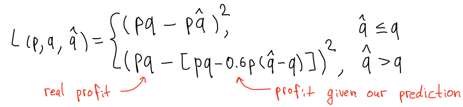
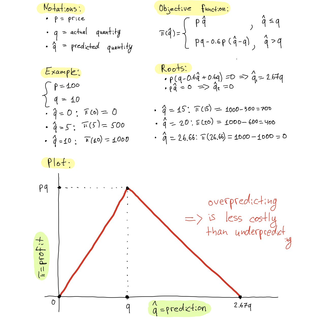
In the DMC 2020 task, we are given a profit function of the retailer. The function accounts for asymmetric error costs: underpredicting demand results in lost revenue because the retailer can not sell a product that is not ready to ship, whereas overpredicting demand incurs a fee for storing the excessive amount of product.

Below, we derive profit according to the task description:

Let's implement the profit function in Python:

def profit(y_true, y_pred, price):
    '''
    Computes retailer's profit.
    
    Arguments:
    - y_true (numpy array): ground truth demand values
    - y_pred (numpy array): predicted demand values
    - price (numpy array): item prices

    Returns:
    - profit value
    '''

    # remove negative and round
    y_pred = np.where(y_pred > 0, y_pred, 0)
    y_pred = np.round(y_pred).astype('int')

    # sold units
    units_sold = np.minimum(y_true, y_pred)

    # overstocked units
    units_overstock = y_pred - y_true
    units_overstock[units_overstock < 0] = 0

    # profit
    revenue = units_sold * price
    fee     = units_overstock * price * 0.6
    profit  = revenue - fee
    profit  = profit.sum()
    
    return profit

The function above is great for evaluating quality of our predictions. But can we directly optimize it during modeling?

LightGBM supports custom loss functions on both training and validation stages. To use a custom loss during training, one needs to supply a function with its first and second-order derivatives.

Ideally, we would like to define the loss as a difference between the potential profit (given our demand prediction) and the oracle profit (when demand prediction is correct). However, such a loss is not differentiable. We can not compute derivatives to plug it as a training loss. Instead, we need to come up with a slightly different function that approximates profit and satisfies the loss conditions.

We define the loss as a squared difference between the oracle profit and profit based on predicted demand. In this setting, we can compute loss derivatives with respect to the prediction (Gradient and Hessian):

The snippet below implements the training and validation losses for LightGBM. You can notice that we do not include the squared prices in the loss functions. The reason is that with sklearn API, it is difficult to include external variables like prices in the loss, so we will include the price later.

# collpase-show

##### TRAINING LOSS
def asymmetric_mse(y_true, y_pred):
    '''
    Asymmetric MSE objective for training LightGBM regressor.
     
    Arguments:
    - y_true (numpy array): ground truth target values
    - y_pred (numpy array): estimated target values
    
    Returns:
    - gradient
    - hessian
    '''
    
    residual = (y_true - y_pred).astype('float')    
    grad     = np.where(residual > 0, -2*residual, -0.72*residual)
    hess     = np.where(residual > 0,  2.0, 0.72)
    return grad, hess


##### VALIDATION LOSS
def asymmetric_mse_eval(y_true, y_pred):
    
    '''
    Asymmetric MSE evaluation metric for evaluating LightGBM regressor.
     
    Arguments:
    - y_true (numpy array): ground truth target values
    - y_pred (numpy array): estimated target values
    
    Returns:
    - metric name
    - metric value
    - whether the metric is maximized
    '''
    
    residual = (y_true - y_pred).astype('float')      
    loss     = np.where(residual > 0, 2*residual**2, 0.72*residual**2)
    return 'asymmetric_mse_eval', np.mean(loss), False

How to deal with the prices?

One option is to account for them within the fit() method. LightGBM supports weighing observations using the arguments sample_weight and eval_sample_weight. You will see how we supply price vectors in the modeling code in the next section. Note that including prices as weights instead of plugging them into the loss leads to losing some information, since Gradients and Hessians are computed without the price multiplication. Still, this approach provides a pretty close approximation of the original profit function. If you are interested in including prices in the loss, you can check lightGBM API that allows more flexibility.

The only missing piece is the relationship between the penalty size and the prediction error. By taking a square root of the profit differences instead of the absolute value, we penalize larger errors more than the smaller ones. However, our profit changes linearly with the error size. This is how we can can address it:

• transform target using a non-linear transformation (e.g. square root)
• train a model that optimizes the MSE loss on the transformed target
• apply the inverse transformation to the model predictions

Target transformation smooths out the square effect in MSE. We still penalize large errors more, but the large errors on a transformed scale are also smaller compared to the original scale. This helps to balance the two effects and approximate a linear relationship between the error size and the loss penalty.

Modeling pipeline

Good, let's start building models! First, we extract the target and flag ID features not used for prediction.

#collapse-hide

# extract target
y = df_train['target']
X = df_train.drop('target', axis = 1)
del df_train
print(X.shape, y.shape)

# format test data
X_test = df_test.drop('target', axis = 1)
del df_test
print(X_test.shape)

# relevant features
drop_feats = ['itemID', 'day_of_year']
features = [var for var in X.columns if var not in drop_feats]

(1381116, 475) (1381116,)
(10463, 475)

The modeling pipeline uses multiple tricks discovered during the model refinement process. We toggle these tricks using logical variables that define the following training options:

• target_transform = True: transforms target to reduce penalty for large errors. Motivation for this is provided in the previous section.
• train_on_positive = False: trains only on cases with positive sales (i.e., at least one of the order lags is greater than zero) and predicts null demand for items with no sales. This substantially reduces the training time but also leads to a drop in the performance.
• two_stage = True: trains a two-stage model: (i) binary classifier predicting whether the future sales will be zero; (ii) regression model predicting the volume of sales. Predictions of the regression model are only stored for cases where the classifier predicts positive sales.
• tuned_params = True: imports optimized LightGBM hyper-parameter values. The next section describes the tuning procedure.

#collapse-hide

##### TRAINING OPTIONS

# target transformation
target_transform = True

# train on positive sales only
train_on_positive = False

# two-stage model
two_stage = True

# use tuned meta-params
tuned_params = True


##### CLASSIFIER PARAMETERS

# rounds and options
cores       = 4
stop_rounds = 100
verbose     = 100
seed        = 23

# LGB parameters
lgb_params = {
    'boosting_type':    'goss',
    'objective':        asymmetric_mse,
    'metrics':          asymmetric_mse_eval,
    'n_estimators':     1000,
    'learning_rate':    0.1,
    'bagging_fraction': 0.8,
    'feature_fraction': 0.8,
    'lambda_l1':        0.1,
    'lambda_l2':        0.1,
    'silent':           True,
    'verbosity':        -1,
    'nthread' :         cores,
    'random_state':     seed,
}

# load optimal parameters
if tuned_params:
    par_file   = open('../lgb_meta_params_100.pkl', 'rb')
    lgb_params = pickle.load(par_file)
    lgb_params['nthread']      = cores
    lgb_params['random_state'] = seed

# second-stage LGB
if two_stage:
    lgb_classifier_params              = lgb_params.copy()
    lgb_classifier_params['objective'] = 'binary'
    lgb_classifier_params['metrics']   = 'logloss'

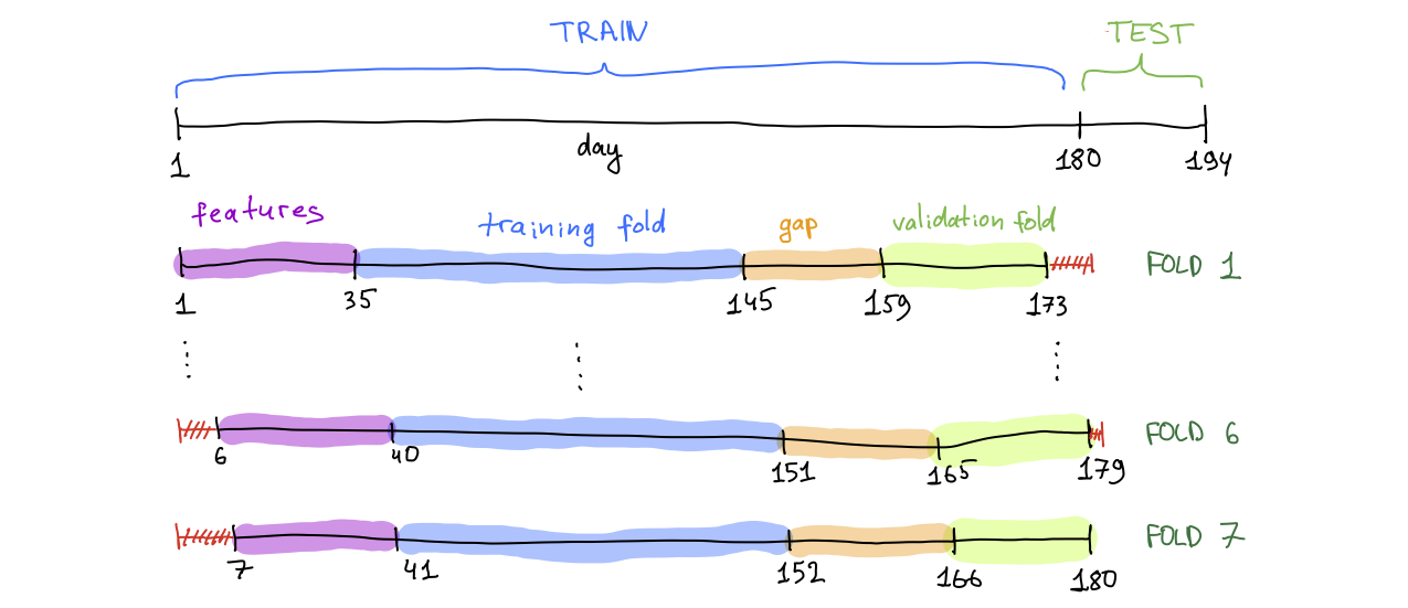
We also define the partitioning parameters. We use a sliding window approach with 7 folds, where each subsequent fold is shifted by one day into the past.

#collapse-hide
num_folds = 7   # no. CV folds
test_days = 14  # no. days in the test set

Let's explain the partitioning using the first fold as an example. Each fold is divided into training and validation subsets. The first 35 days are cut off and only used to compute lag-based features for the days starting from 36. Days 36 - 145 are used for training. For each of these days, we have features based on the previous 35 days and targets based on the next 14 days. Days 159 - 173 are used for validation. Days 146 - 158 between training and validation subsets are skipped to avoid data leakage: the target for these days would use information from the validation period.

We can now set up a modeling loop with the following steps for each of the folds:

• extract data from the fold and partition it into training and validation sets
• train LightGBM on the training set and perform early stopping on the validation set
• save predictions for the validation set (denoted as OOF) and predictions for the test set
• save feature importance and performance on the validation fold

#collapse-show

# placeholders
importances   = pd.DataFrame()
preds_oof     = np.zeros((num_folds, items.shape[0]))
reals_oof     = np.zeros((num_folds, items.shape[0]))
prices_oof    = np.zeros((num_folds, items.shape[0]))
preds_test    = np.zeros(items.shape[0])
oof_rmse      = []
oof_profit    = []
oracle_profit = []
clfs          = []
train_idx     = []
valid_idx     = []

# objects
train_days = X['day_of_year'].max() - test_days + 1 - num_folds - X['day_of_year'].min() # no. days in the train set
time_start = time.time()

# modeling loop
for fold in range(num_folds):
    
    ##### PARTITIONING
    
    # dates
    if fold == 0:
        v_end = X['day_of_year'].max()
    else:
        v_end = v_end - 1
    v_start = v_end
    t_end   = v_start - (test_days + 1)
    t_start = t_end   - (train_days - 1)
    
    # extract index
    train_idx.append(list(X[(X.day_of_year >= t_start) & (X.day_of_year <= t_end)].index))
    valid_idx.append(list(X[(X.day_of_year >= v_start) & (X.day_of_year <= v_end)].index))   
    
    # extract samples
    X_train, y_train = X.iloc[train_idx[fold]][features], y.iloc[train_idx[fold]]
    X_valid, y_valid = X.iloc[valid_idx[fold]][features], y.iloc[valid_idx[fold]]
    X_test = X_test[features]
    
    # keep positive cases
    if train_on_positive:
        y_train = y_train.loc[(X_train['order_sum_last_28'] > 0) | (X_train['promo_in_test'] > 0)]
        X_train = X_train.loc[(X_train['order_sum_last_28'] > 0) | (X_train['promo_in_test'] > 0)]

    # information
    print('-' * 65)
    print('- train period days: {} -- {} (n = {})'.format(t_start, t_end, len(train_idx[fold])))
    print('- valid period days: {} -- {} (n = {})'.format(v_start, v_end, len(valid_idx[fold])))
    print('-' * 65)

    
    ##### MODELING
    
    # target transformation
    if target_transform:
        y_train = np.sqrt(y_train)
        y_valid = np.sqrt(y_valid)
        
    # first stage model
    if two_stage:
        y_train_binary, y_valid_binary = y_train.copy(), y_valid.copy()
        y_train_binary[y_train_binary > 0] = 1
        y_valid_binary[y_valid_binary > 0] = 1
        clf_classifier = lgb.LGBMClassifier(**lgb_classifier_params) 
        clf_classifier = clf_classifier.fit(X_train, y_train_binary, 
                                            eval_set              = [(X_train, y_train_binary), (X_valid, y_valid_binary)],
                                            eval_metric           = 'logloss',
                                            early_stopping_rounds = stop_rounds,
                                            verbose               = verbose)
        preds_oof_fold_binary  = clf_classifier.predict(X_valid)
        preds_test_fold_binary = clf_classifier.predict(X_test)

    # training
    clf = lgb.LGBMRegressor(**lgb_params) 
    clf = clf.fit(X_train, y_train, 
                  eval_set              = [(X_train, y_train), (X_valid, y_valid)], 
                  eval_metric           = asymmetric_mse_eval,
                  sample_weight         = X_train['simulationPrice'].values,
                  eval_sample_weight    = [X_train['simulationPrice'].values, X_valid['simulationPrice'].values],
                  early_stopping_rounds = stop_rounds,
                  verbose               = verbose)
    clfs.append(clf)
    
    # inference
    if target_transform:      
        preds_oof_fold  = postprocess_preds(clf.predict(X_valid)**2)
        reals_oof_fold  = y_valid**2
        preds_test_fold = postprocess_preds(clf.predict(X_test)**2) / num_folds
    else:
        preds_oof_fold  = postprocess_preds(clf.predict(X_valid))
        reals_oof_fold  = y_valid
        preds_test_fold = postprocess_preds(clf.predict(X_test)) / num_folds
        
    # impute zeros
    if train_on_positive:
        preds_oof_fold[(X_valid['order_sum_last_28'] == 0) & (X_valid['promo_in_test'] == 0)] = 0
        preds_test_fold[(X_test['order_sum_last_28'] == 0) & (X_test['promo_in_test']  == 0)] = 0
        
    # multiply with first stage predictions
    if two_stage:
        preds_oof_fold  = preds_oof_fold  * np.round(preds_oof_fold_binary)
        preds_test_fold = preds_test_fold * np.round(preds_test_fold_binary)

    # write predictions
    preds_oof[fold, :] = preds_oof_fold
    reals_oof[fold, :] = reals_oof_fold
    preds_test        += preds_test_fold
    
    # save prices
    prices_oof[fold, :] = X.iloc[valid_idx[fold]]['simulationPrice'].values
        
        
    ##### EVALUATION

    # evaluation
    oof_rmse.append(np.sqrt(mean_squared_error(reals_oof[fold, :], 
                                               preds_oof[fold, :])))
    oof_profit.append(profit(reals_oof[fold, :], 
                             preds_oof[fold, :], 
                             price = X.iloc[valid_idx[fold]]['simulationPrice'].values))
    oracle_profit.append(profit(reals_oof[fold, :], 
                                reals_oof[fold, :], 
                                price = X.iloc[valid_idx[fold]]['simulationPrice'].values))
    
    # feature importance
    fold_importance_df = pd.DataFrame()
    fold_importance_df['Feature'] = features
    fold_importance_df['Importance'] = clf.feature_importances_
    fold_importance_df['Fold'] = fold + 1
    importances = pd.concat([importances, fold_importance_df], axis = 0)
    
    # information
    print('-' * 65)
    print('FOLD {:d}/{:d}: RMSE = {:.2f}, PROFIT = {:.0f}'.format(fold + 1, 
                                                                  num_folds, 
                                                                  oof_rmse[fold], 
                                                                  oof_profit[fold]))
    print('-' * 65)
    print('')
    

# print performance
print('')
print('-' * 65)
print('- AVERAGE RMSE:   {:.2f}'.format(np.mean(oof_rmse)))
print('- AVERAGE PROFIT: {:.0f} ({:.2f}%)'.format(np.mean(oof_profit), 100 * np.mean(oof_profit) / np.mean(oracle_profit)))
print('- RUNNING TIME:   {:.2f} minutes'.format((time.time() - time_start) / 60))
print('-' * 65)

-----------------------------------------------------------------
- train period days: 41 -- 151 (n = 1161393)
- valid period days: 166 -- 166 (n = 10463)
-----------------------------------------------------------------
Training until validation scores don't improve for 100 rounds
Early stopping, best iteration is:
[532]	training's binary_logloss: 0.238417	valid_1's binary_logloss: 0.347182
Training until validation scores don't improve for 100 rounds
Early stopping, best iteration is:
[788]	training's rmse: 0.611924	training's asymmetric_mse_eval: 2.82734	valid_1's rmse: 0.98004	valid_1's asymmetric_mse_eval: 5.83945
-----------------------------------------------------------------
FOLD 1/7: RMSE = 74.46, PROFIT = 4146664
-----------------------------------------------------------------

...

-----------------------------------------------------------------
- train period days: 35 -- 145 (n = 1161393)
- valid period days: 160 -- 160 (n = 10463)
-----------------------------------------------------------------
Training until validation scores don't improve for 100 rounds
Early stopping, best iteration is:
[711]	training's binary_logloss: 0.22193	valid_1's binary_logloss: 0.338637
Training until validation scores don't improve for 100 rounds
Early stopping, best iteration is:
[782]	training's rmse: 0.600011	training's asymmetric_mse_eval: 2.71385	valid_1's rmse: 0.987073	valid_1's asymmetric_mse_eval: 5.67223
-----------------------------------------------------------------
FOLD 7/7: RMSE = 74.46, PROFIT = 3958098
-----------------------------------------------------------------


-----------------------------------------------------------------
- AVERAGE RMSE:   69.66
- AVERAGE PROFIT: 3997598 (54.19%)
- RUNNING TIME:   88.53 minutes
-----------------------------------------------------------------

Looks good! The modeling pipeline took us about 1.5 hours to run.

Forecasting demand with our models results in 3,997,598 daily profit, which is about 54% of the maximum possible profit. Let's visualize the results:

# collapse-hide

fig = plt.figure(figsize = (20, 7))

# residual plot
plt.subplot(1, 2, 1)
plt.scatter(reals_oof.reshape(-1), preds_oof.reshape(-1))
axis_lim = np.max([reals_oof.max(), preds_oof.max()])
plt.ylim(top   = 1.02*axis_lim)
plt.xlim(right = 1.02*axis_lim)
plt.plot((0, axis_lim), (0, axis_lim), 'r--')
plt.title('Residual Plot')
plt.ylabel('Predicted demand')
plt.xlabel('Actual demand')

# feature importance
plt.subplot(1, 2, 2)
top_feats = 50
cols = importances[['Feature', 'Importance']].groupby('Feature').mean().sort_values(by = 'Importance', ascending = False)[0:top_feats].index
importance = importances.loc[importances.Feature.isin(cols)]
sns.barplot(x = 'Importance', y = 'Feature', data = importance.sort_values(by = 'Importance', ascending = False), ci = 0)
plt.title('Feature Importance')
plt.tight_layout()

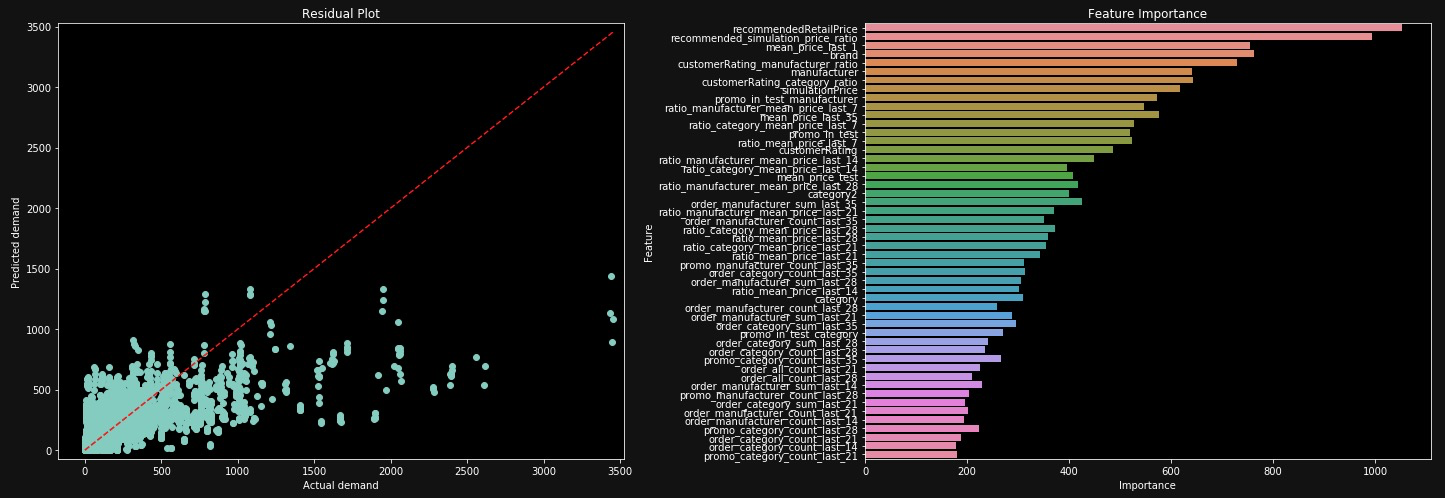
The scatterplot shows that there is a space for further improvement: many predictions are far from the 45-degree line where predicted and real orders are equal. The important features mostly contain price information followed by features that count the previous orders.

We can now use predictions stored in preds_test to create a submission. Mission accomplished!

5. Hyper-parameter tuning

One way to improve our solution is to optimize the LightGBM hyper-parameters.

We tune hyper-parameters using the hyperopt package, which performs optimization using Tree of Parzen Estimators (TPE) as a search algorithm. You don't really need to know how TPE works. As a user, you are only required to supply a parameter grid indicating the range of possible values. Compared to standard tuning methods like grid search or random search, TPE explores the search space more efficiently, allowing you to find a suitable solution faster. If you want to read more, see the package documentation here.

So, let's specify hyper-parameter ranges! We create a dictionary using the following options:

• hp.choice('name', list_of_values): sets a hyper-parameter to one of the values from a list. This is suitable for hyper-parameters that can have multiple distinct values like boosting_type
• hp.uniform('name', min, max): sets a hyper-parameter to a float between min and max. This works well with hyper-parameters such as learning_rate
• hp.quniform('name', min, max, step): sets a hyper-parameter to a value between min and max with a step size of step. This is useful for integer parameters like max_depth

#collapse-show

# training params
lgb_reg_params = {    
    'boosting_type':    hp.choice('boosting_type', ['gbdt', 'goss']),    
    'objective':        'rmse',
    'metrics':          'rmse',
    'n_estimators':     10000,
    'learning_rate':    hp.uniform('learning_rate',  0.0001, 0.3),
    'max_depth':        hp.quniform('max_depth',          1,  16, 1),
    'num_leaves':       hp.quniform('num_leaves',        10,  64, 1),
    'bagging_fraction': hp.uniform('bagging_fraction',  0.3,   1),
    'feature_fraction': hp.uniform('feature_fraction',  0.3,   1),
    'lambda_l1':        hp.uniform('lambda_l1',           0,   1),
    'lambda_l2':        hp.uniform('lambda_l2',           0,   1),
    'silent':           True,
    'verbosity':        -1,
    'nthread' :         4,
    'random_state':     77,
}

# evaluation params
lgb_fit_params = {
    'eval_metric':           'rmse',
    'early_stopping_rounds': 100,
    'verbose':               False,
}

# combine params
lgb_space = dict()
lgb_space['reg_params'] = lgb_reg_params
lgb_space['fit_params'] = lgb_fit_params

Next, we create HPOpt object that performs tuning. We can avoid this in a simple tuning task, but defining an object gives us more control of the optimization process, which is useful with a custom loss. We define three object methods:

• process: runs optimization. By default, HPO uses fmin() to minimize the specified loss
• lgb_reg: initializes LightGBM model
• train_reg: trains LightGBM and computes the loss. Since we aim to maximize profit, we simply define loss as negative profit

# collapse-show
class HPOpt(object):

    # INIT
    def __init__(self, x_train, x_test, y_train, y_test):
        self.x_train = x_train
        self.x_test  = x_test
        self.y_train = y_train
        self.y_test  = y_test

    # optimization process
    def process(self, fn_name, space, trials, algo, max_evals):
        fn = getattr(self, fn_name)
        try:
            result = fmin(fn        = fn, 
                          space     = space, 
                          algo      = algo, 
                          max_evals = max_evals, 
                          trials    = trials)
        except Exception as e:
            return {'status': STATUS_FAIL, 'exception': str(e)}
        return result, trials
    
    
    # LGBM initialization
    def lgb_reg(self, para):
        para['reg_params']['max_depth']  = int(para['reg_params']['max_depth'])
        para['reg_params']['num_leaves'] = int(para['reg_params']['num_leaves'])
        reg = lgb.LGBMRegressor(**para['reg_params'])
        return self.train_reg(reg, para)

    
    # training and inference
    def train_reg(self, reg, para):
        
        # fit LGBM
        reg.fit(self.x_train, self.y_train,
                eval_set              = [(self.x_train, self.y_train), (self.x_test, self.y_test)], 
                sample_weight         = self.x_train['simulationPrice'].values,
                eval_sample_weight    = [self.x_train['simulationPrice'].values, self.x_test['simulationPrice'].values],
                **para['fit_params'])
        
        # inference
        if target_transform:      
            preds = postprocess_preds(reg.predict(self.x_test)**2)
            reals = self.y_test**2
        else:
            preds = postprocess_preds(reg.predict(self.x_test))
            reals = self.y_test

        # compute loss [negative profit]
        loss = np.round(-profit(reals, preds, price = self.x_test['simulationPrice'].values))
                      
        return {'loss': loss, 'status': STATUS_OK}

To prevent overfitting, we perform tuning on a different subset of data compared to the models trained in the previous section by going one day further in the past.

# collapse-hide

# validation dates
v_end   = 158          # 1 day before last validation fold in code_03_modeling
v_start = v_end        # same as v_start

# training dates
t_start = 28           # first day in the data
t_end   = v_start - 15 # validation day - two weeks

# extract index
train_idx = list(X[(X.day_of_year >= t_start) & (X.day_of_year <= t_end)].index)
valid_idx = list(X[(X.day_of_year >= v_start) & (X.day_of_year <= v_end)].index)   

# extract samples
X_train, y_train = X.iloc[train_idx][features], y.iloc[train_idx]
X_valid, y_valid = X.iloc[valid_idx][features], y.iloc[valid_idx]
    
# target transformation
if target_transform:
    y_train = np.sqrt(y_train)
    y_valid = np.sqrt(y_valid)

# information
print('-' * 65)
print('- train period days: {} -- {} (n = {})'.format(t_start, t_end, len(train_idx)))
print('- valid period days: {} -- {} (n = {})'.format(v_start, v_end, len(valid_idx)))
print('-' * 65)

-----------------------------------------------------------------
- train period days: 28 -- 143 (n = 1213708)
- valid period days: 158 -- 158 (n = 10463)
-----------------------------------------------------------------

Now, we just need to instantiate the HPOpt object and launch the tuning trials! The optimization will run automatically, and we would only need to extract the optimized values:

# collapse-show

# instantiate objects
hpo_obj = HPOpt(X_train, X_valid, y_train, y_valid)
trials  = Trials() 

# perform tuning
lgb_opt_params = hpo_obj.process(fn_name   = 'lgb_reg',
                                 space     = lgb_space, 
                                 trials    = trials, 
                                 algo      = tpe.suggest, 
                                 max_evals = tuning_trials)  

# merge best params to fixed params
params = list(lgb_opt_params[0].keys())
for par_id in range(len(params)):
    lgb_reg_params[params[par_id]] = lgb_opt_params[0][params[par_id]]
    
# postprocess
lgb_reg_params['boosting_type'] = boost_types[lgb_reg_params['boosting_type']]
lgb_reg_params['max_depth']     = int(lgb_reg_params['max_depth'])
lgb_reg_params['num_leaves']    = int(lgb_reg_params['num_leaves'])

# print best params
print('Best meta-parameters:')
lgb_reg_params

Best meta-parameters:

{'boosting_type': 'goss',
 'objective': 'rmse',
 'metrics': 'rmse',
 'n_estimators': 10000,
 'learning_rate': 0.004012,
 'max_depth': 10,
 'num_leaves': 64,
 'bagging_fraction': 0.934688,
 'feature_fraction': 0.668076,
 'lambda_l1': 0.280133,
 'lambda_l2': 0.589682,
 'silent': True,
 'verbosity': -1,
 'nthread': 4,
 'random_state': 77}

Done! Now we can save the optimized values and import them when setting up the model.

# collapse-hide
par_file = open('../lgb_meta_params.pkl', 'wb')
pickle.dump(lgb_reg_params, par_file)
par_file.close()

6. Closing words

This blog post has finally come to an end. Thank you for reading!

We looked at important stages of our solution and covered steps such as data aggregation, feature engineering, custom loss functions, target transformation and hyper-parameter tuning.

Our final solution was a simple ensemble of multiple LightGBM models with different features and training options discussed in this post. If you are interested in the ensembling part, you can find the codes in my Github.

Please feel free to use the comment window below to ask questions and stay tuned for the next editions of Data Mining Cup!