Gradient Accumulation in PyTorch
Increasing batch size to overcome memory constraints


Last update: 15.10.2021
1. Overview
Deep learning models are getting bigger and bigger. It becomes difficult to fit such networks in the GPU memory. This is especially relevant in computer vision applications where we need to reserve some memory for high-resolution images as well. As a result, we are sometimes forced to use small batches during training, which may lead to a slower convergence and lower accuracy.
This blog post provides a quick tutorial on how to increase the effective batch size by using a trick called gradient accumulation. Simply speaking, gradient accumulation means that we will use a small batch size but save the gradients and update network weights once every couple of batches. Automated solutions for this exist in higher-level frameworks such as fast.ai or lightning, but those who love using PyTorch might find this tutorial useful.
2. What is gradient accumulation
When training a neural network, we usually divide our data in mini-batches and go through them one by one. The network predicts batch labels, which are used to compute the loss with respect to the actual targets. Next, we perform backward pass to compute gradients and update model weights in the direction of those gradients.
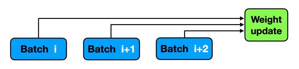
Gradient accumulation modifies the last step of the training process. Instead of updating the network weights on every batch, we can save gradient values, proceed to the next batch and add up the new gradients. The weight update is then done only after several batches have been processed by the model.
Gradient accumulation helps to imitate a larger batch size. Imagine you want to use 32 images in one batch, but your hardware crashes once you go beyond 8. In that case, you can use batches of 8 images and update weights once every 4 batches. If you accumulate gradients from every batch in between, the results will be (almost) the same and you will be able to perform training on a less expensive machine!
# loop through batches
for (inputs, labels) in data_loader:

    # extract inputs and labels
    inputs = inputs.to(device)
    labels = labels.to(device)

    # passes and weights update
    with torch.set_grad_enabled(True):

        # forward pass
        preds = model(inputs)
        loss  = criterion(preds, labels)

        # backward pass
        loss.backward()

        # weights update
        optimizer.step()
        optimizer.zero_grad()
Now let's implement gradient accumulation! There are three things we need to do:
- Specify the
accum_iterparameter. This is just an integer value indicating once in how many batches we would like to update the network weights. - Condition the weight update on the index of the running batch. This requires using
enumerate(data_loader)to store the batch index when looping through the data. - Divide the running loss by
acum_iter. This normalizes the loss to reduce the contribution of each mini-batch we are actually processing. Depending on the way you compute the loss, you might not need this step: if you average loss within each batch, the division is already correct and there is no need for extra normalization.
# batch accumulation parameter
accum_iter = 4

# loop through enumaretad batches
for batch_idx, (inputs, labels) in enumerate(data_loader):

    # extract inputs and labels
    inputs = inputs.to(device)
    labels = labels.to(device)

    # passes and weights update
    with torch.set_grad_enabled(True):

        # forward pass
        preds = model(inputs)
        loss  = criterion(preds, labels)

        # normalize loss to account for batch accumulation
        loss = loss / accum_iter

        # backward pass
        loss.backward()

        # weights update
        if ((batch_idx + 1) % accum_iter == 0) or (batch_idx + 1 == len(data_loader)):
            optimizer.step()
            optimizer.zero_grad()
It is really that simple! The gradients are computed when we call loss.backward() and are stored by PyTorch until we call optimizer.zero_grad(). Therefore, we just need to move the weight update performed in optimizer.step() and the gradient reset under the if condition that check the batch index. It is important to also update weights on the last batch when batch_idx + 1 == len(data_loader) - this makes sure that data from the last batches are not discarded and used for optimizing the network.
Please also note that some network architectures have batch-specific operations. For instance, batch normalization is performed on a batch level and therefore may yield slightly different results when using the same effective batch size with and without gradient accumulation. This means that you should not expect to see a 100% match between the results.
In my experience, the potential performance gains from increasing the number of cases used to update the network weights are largest when one is forced to use very small batches (e.g., 8 or 10). Therefore, I always recommend using gradient accumulation when working with large architectures that consume a lof of GPU memory.
Liked the post? Share it on social media!
You can also buy me a cup of tea to support my work. Thanks!
