Computing Mean & STD in Image Dataset
How to get channel-speicific mean and std in PyTorch


Last update: 16.10.2021
1. Overview
In computer vision, it is recommended to normalize image pixel values relative to the dataset mean and standard deviation. This helps to get consistent results when applying a model to new images and can also be useful for transfer learning. In practice, computing these statistics can be a little non-trivial since we usually can't load the whole dataset in memory and have to loop through it in batches.
This blog post provides a quick tutorial on computing dataset mean and std within RGB channels using a regular PyTorch dataloader. While computing mean is easy (we can simply average means over batches), standard deviation is a bit more tricky: averaging STDs across batches is not the same as the overall STD. Let's see how to do it properly!
2. Preparations
To demonstrate how to compute image stats, we will use data from Cassava Leaf Disease Classification Kaggle competition with about 21,000 plant images. Feel free to scroll down to Section 3 to jump directly to calculations.
First, we will import the usual libraries and specify relevant parameters. No need to use GPU because there is no modeling involved.
#collapse-hide

####### PACKAGES

import numpy as np
import pandas as pd

import torch
import torchvision
from torch.utils.data import Dataset, DataLoader

import albumentations as A
from albumentations.pytorch import ToTensorV2

import cv2

from tqdm import tqdm

import matplotlib.pyplot as plt
%matplotlib inline


####### PARAMS

device      = torch.device('cpu')
num_workers = 4
image_size  = 512
batch_size  = 8
data_path   = '/kaggle/input/cassava-leaf-disease-classification/'
Now, let's import a dataframe with image paths and create a Dataset class that will read images and supply them to the dataloader.
#collapse-show

df = pd.read_csv(data_path + 'train.csv')
df.head()
#collapse-show

class LeafData(Dataset):

    def __init__(self,
                 data,
                 directory,
                 transform = None):
        self.data      = data
        self.directory = directory
        self.transform = transform

    def __len__(self):
        return len(self.data)

    def __getitem__(self, idx):

        # import
        path  = os.path.join(self.directory, self.data.iloc[idx]['image_id'])
        image = cv2.imread(path, cv2.COLOR_BGR2RGB)

        # augmentations
        if self.transform is not None:
            image = self.transform(image = image)['image']

        return image
We want to compute stats for raw images, so our data augmentation pipeline should be minimal and not include any heavy transformations we might use during training. Below, we use A.Normalize() with mean = 0 and std = 1 to scale pixel values from [0, 255] to [0, 1] and ToTensorV2() to convert numpy arrays into torch tensors.
#collapse-show

augs = A.Compose([A.Resize(height = image_size,
                           width  = image_size),
                  A.Normalize(mean = (0, 0, 0),
                              std  = (1, 1, 1)),
                  ToTensorV2()])
Let's check if our code works correctly. We define a DataLoader to load images in batches from LeafData and plot the first batch.
####### EXAMINE SAMPLE BATCH

# dataset
image_dataset = LeafData(data      = df,
                         directory = data_path + 'train_images/',
                         transform = augs)

# data loader
image_loader = DataLoader(image_dataset,
                          batch_size  = batch_size,
                          shuffle     = False,
                          num_workers = num_workers,
                          pin_memory  = True)

# display images
for batch_idx, inputs in enumerate(image_loader):
    fig = plt.figure(figsize = (14, 7))
    for i in range(8):
        ax = fig.add_subplot(2, 4, i + 1, xticks = [], yticks = [])
        plt.imshow(inputs[i].numpy().transpose(1, 2, 0))
    break

Looks like everithing is working correctly! Now we can use our image_loader to compute image stats.
3. Computing image stats
The computation is done in three steps:
- Define placeholders to store two batch-level stats: sum and squared sum of pixel values. The first will be used to compute means, and the latter will be needed for standard deviation calculations.
- Loop through the batches and add up channel-specific sum and squared sum values.
- Perform final calculations to obtain data-level mean and standard deviation.
The first two steps are done in the snippet below. Note that we set axis = [0, 2, 3] to compute mean values with respect to axis 1. The dimensions of inputs is [batch_size x 3 x image_size x image_size], so we need to make sure we aggregate values per each RGB channel separately.
####### COMPUTE MEAN / STD

# placeholders
psum    = torch.tensor([0.0, 0.0, 0.0])
psum_sq = torch.tensor([0.0, 0.0, 0.0])

# loop through images
for inputs in tqdm(image_loader):
    psum    += inputs.sum(axis        = [0, 2, 3])
    psum_sq += (inputs ** 2).sum(axis = [0, 2, 3])
Finally, we make some further calculations:
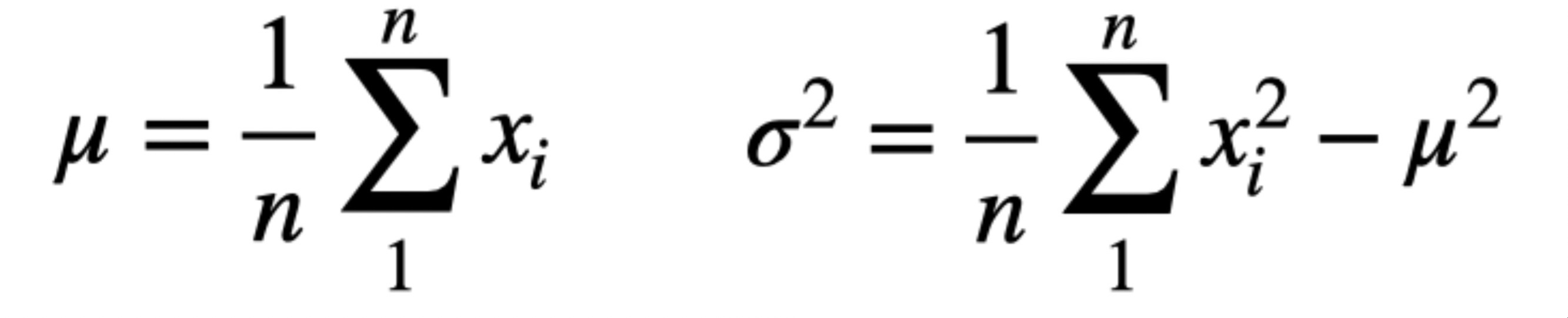
- mean: simply divide the sum of pixel values by the total
count- number of pixels in the dataset computed aslen(df) * image_size * image_size - standard deviation: use the following equation:
total_std = sqrt(psum_sq / count - total_mean ** 2)
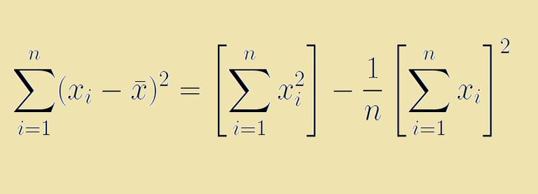
Why we use such a weird formula for STD? Well, because this is how the variance equation can be simplified to make use of the sum of squares when other data is not available. If you are not sure about this, expand the cell below to see a calculation example or read this for some details.
#collapse-hide

# Consider three vectors:
A = [1, 1]
B = [2, 2]
C = [1, 1, 2, 2]

# Let's compute SDs in a classical way:
1. Mean(A) = 1; Mean(B) = 2; Mean(C) = 1.5
2. SD(A) = SD(B) = 0  # because there is no variation around the means
3. SD(C) = sqrt(1/4 * ((1 - 1.5)**2 + (1 - 1.5)**2 + (1 - 1.5)**2 + (1 - 1.5)**2)) = 1/2

# Note that SD(C) is clearly not equal to SD(A) + SD(B), which is zero.

# Instead, we could compute SD(C) in three steps using the equation above:
1. psum    = 1 + 1 + 2 + 2 = 6
2. psum_sq = (1**2 + 1**2 + 2**2 + 2**2) = 10
3. SD(C)   = sqrt((psum_sq - 1/N * psum**2) / N) = sqrt((10 - 36 / 4) / 4) = sqrt(1/4) = 1/2

# We get the same result as in the classical way!
####### FINAL CALCULATIONS

# pixel count
count = len(df) * image_size * image_size

# mean and std
total_mean = psum / count
total_var  = (psum_sq / count) - (total_mean ** 2)
total_std  = torch.sqrt(total_var)

# output
print('mean: '  + str(total_mean))
print('std:  '  + str(total_std))
This is it! Now you can plug in the mean and std values to A.Normalize() in your data augmentation pipeline to make sure your dataset is normalized :)
4. Closing words
I hope this tutorial was helpful for those looking for a quick guide on computing the image dataset stats. From my experience, normalizing images with respect to the data-level mean and std does not always help to improve the performance, but it is one of the things I always try first. Happy learning and stay tuned for the next posts!
Liked the post? Share it on social media!
You can also buy me a cup of tea to support my work. Thanks!
